Understand the fitness landscape of your optimization problem.

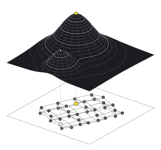
A fitness landscape maps the candidates in a design space, such as protein variants or reaction conditions, to their measured performance. GraphFLA builds this landscape from your data and characterizes its topography, revealing what makes a problem easy or hard to model and to optimize. These insights help you develop better predictive models and search algorithms.

Get started
$ pip install graphfla
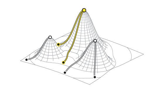
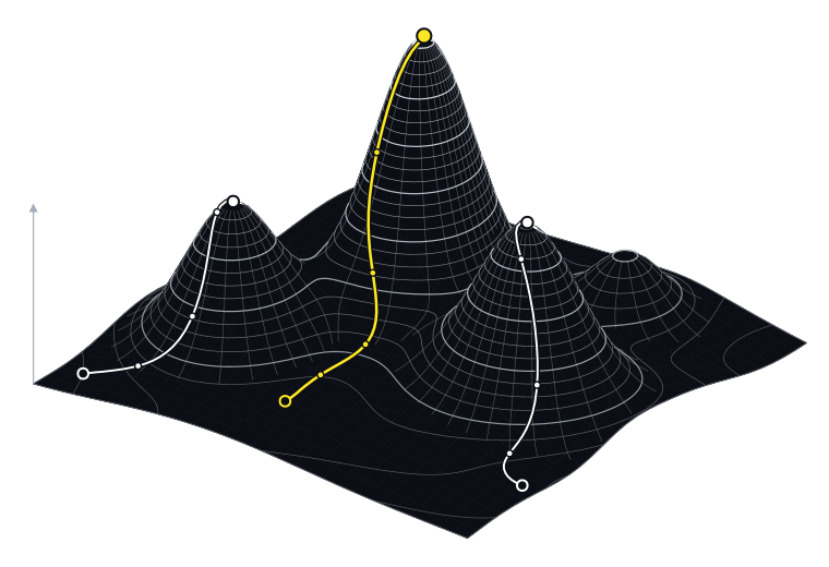
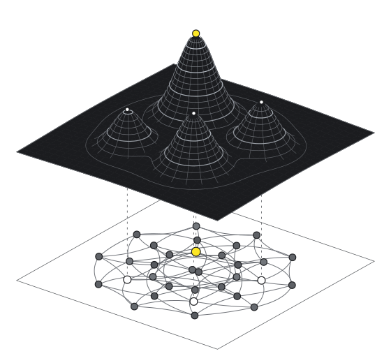
An illustrative fitness landscape with improving paths, one reaching the global optimum and two ending at local optima. Global optimum Local optimum Local optimum fitness design space
  • improving path to the global optimum
  • improving paths ending at local optima

20+

measures of landscape structure

7

landscape types for sequences, categorical, ordinal and mixed data

8

model landscapes and benchmark problems

9

step-by-step tutorials on published data

179

curated datasets from biology, chemistry and materials science

How it works

Build, analyze, and manipulate fitness landscapes as graphs.

Illustrative data and profiles

Enzyme activity

Change amino acids at three sites to improve enzyme activity.

1Provide your data

A table of tested candidates, with one column for each variable and one for the measured property.

Your data

Protein sequenceActivity
MKTAYIAKQRQISFVKSHFS 23%
MKTAFIAKQRQISFVKSHFS 41%
MKTAYIGKQRQISFVKSHFS 36%
MKTAYIAKQKQISFVKSHFS 57%
MKTAFIGKQRQISFVKSHFS 42%
MKTAFIAKQKQISFVKSHFS 64%
MKTAYIGKQKQISFVKSHFS 73%
MKTAFIGKQKQISFVKSHFS 91%

2Build the landscape

GraphFLA links candidates that are adjacent in the design space, e.g., protein variants that differ by one amino-acid substitution, or reaction conditions that differ by one solvent.

GraphFLA

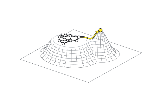
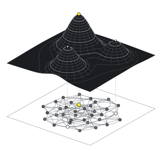
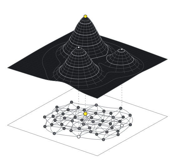
Illustrative enzyme activity landscape with 4 peaks, drawn above its neighbor graph of 32 candidates. Landscape Neighbor graph

3Analyze its topography

Quantify peaks, ruggedness, neutrality and variable interactions.

Landscape profile

Local optima4 / 32

Roughness0.68

Neutrality19%

Fitness-distance correlation−0.25

Variable interactions

  • Magnitude 52%
  • Sign 31%
  • Reciprocal sign 17%

Quick start

From raw data to landscape analysis in a few lines.

Simply load your dataset, specify the variables and the objective, and build the landscape. The same steps apply to laboratory measurements, simulations and model evaluations.

$ pip install graphfla
quickstart.pyPython
import pandas as pdfrom graphfla import analysisfrom graphfla.landscape import ProteinLandscape df = pd.read_csv("variants.csv")X = df["sequence"]  # Amino-acid sequence of each variantf = df["activity"]  # Measured activity, to maximize landscape = ProteinLandscape(maximize=True)landscape.build_from_data(X, f)analysis.profile(landscape, seed=42)

What you can measure

A holistic picture of your landscape, with 20+ features across four aspects.

Each feature is implemented from established studies in evolutionary biology and optimization. Together they let you explore your problem from complementary angles and understand it fully.

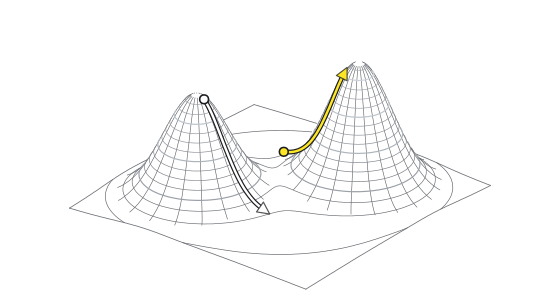
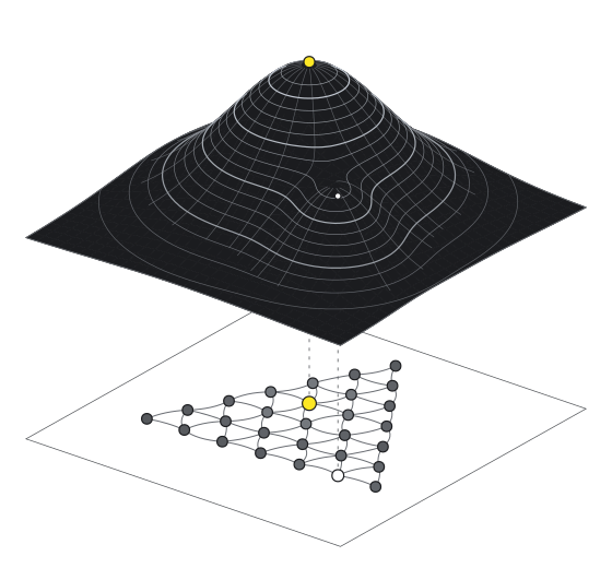
The same change increases fitness in one part of the landscape and decreases it in another.
  • a change that increases fitness here
  • the same change decreases it there

Interactions

Do the variables act independently?

Variables interact when the effect of changing one depends on the values of others, known as epistasis in biology. Interactions that reverse the direction of an effect can block improving paths and create multiple peaks.

Explore interactions

Why landscape topography matters

Landscape features help interpret model performance and optimization outcomes.

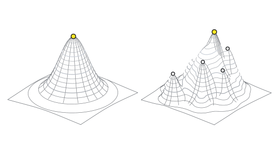
Landscape features help explain why a predictive model or a search method works well on some problems but not on others. In the protein datasets below, compare each feature with the accuracy of zero-shot predictors and with the results of simulated directed evolution.

Zero-shot prediction

ProteinGym · Prediction performance across protein assays

Each point is a protein DMS dataset. Select a landscape feature and a zero-shot model to compare Spearman prediction performance. Use arrow keys to move between points and Enter to read the associated publication. Spearman correlation

Directed evolution

Up to 480 evaluations · 10 runs per landscape

Each point is a protein landscape. Select a feature and a search strategy to compare optimization outcomes within a shared evaluation cap. Use arrow keys to move between points and Enter to read the associated publication. Best fitness percentile

Performance

Scales to millions of candidates on a single machine.

Every stage of landscape construction has been optimized in detail. The comparison below measures construction time and peak memory against a naive implementation that compares all pairs of candidates.

59,161×

faster construction at 1,048,576 candidates

2,384×

lower peak memory on the same build

  • GraphFLA
  • Naive all-pairs

Construction time · log scale

0.1 ms 1 ms 1 s 1 min 1 h 1 day 1 week 256 4,096 65,536 1,048,576 candidates 22 ms 3.6 ms 5.41 s 20 ms 28.5 min 441 ms 6.3 days 9.23 s

Peak memory · log scale

10 MiB 100 MiB 1 GiB 10 GiB 100 GiB 1 TiB 10 TiB 256 4,096 65,536 1,048,576 candidates both 104 MiB 239 MiB 109 MiB 32.3 GiB 280 MiB 8.0 TiB 3.4 GiB

Complete binary landscapes with 8 to 20 variables. Apple M4 Pro, Python 3.9, single thread. Peak memory includes Python and its dependencies. The baseline is a nested Python loop with a dense distance matrix.

Case studies

Applicable to any combinatorial optimization problem.

GraphFLA makes no assumption about what the variables or the objective represent. The same analysis applies to amino acids and reaction conditions, alloy compositions and neural architectures, drug doses and compiler flags.

Suzuki–Miyaura coupling

Chemical reaction optimization

Ligand, base and solvent for one pair of reactants, scored by the UV signal of the coupling product.

384 reaction conditions

Electrochemical flow hydrogenation

Reaction process optimization

Concentration, temperature and residence time in a flow reactor, scored by selectivity and current efficiency.

54 operating conditions

Tungsten–rhenium–osmium alloys

Alloy composition optimization

Tungsten, rhenium and osmium fractions of an alloy, scored by hardness at 1,000 °C.

496 alloy compositions

Hybrid perovskites · ABX₃

Materials design

Organic ion, metal and halide of a hybrid perovskite crystal, scored by its calculated electronic band gap.

192 crystal compositions

BacPUS · Gut bacteria and polysaccharides

Microbial growth optimization

Pairs of gut bacterial strains and polysaccharide nutrient sources, scored by growth after 48 hours.

560 strain–substrate pairs

Cyanimide library · Mouse USP18

Enzyme inhibitor discovery

Amine and carboxylic-acid building blocks combined into inhibitors, scored by inhibition of mouse USP18.

7,504 building-block pairs

NCI-ALMANAC · Cancer cell assays

Drug combination optimization

A partner drug for a fixed anticancer drug and the doses of both, scored by their effect on cancer-cell growth.

900 drug–dose combinations

NAS-Bench-201 · CIFAR-10

Neural architecture search

The operation on each of six connections in a neural-network cell, scored by image-classification accuracy.

15,625 network architectures

LLVM · Compiler flags

Software configuration tuning

Ten LLVM compiler options switched on or off, scored by compilation time for a fixed workload.

1,024 compiler configurations

Analyze your own data.

Research behind GraphFLA

NeurIPS 2025 · Spotlight

Augmenting Biological Fitness Prediction Benchmarks with Landscapes Features from GraphFLA

Mingyu Huang, Shasha Zhou, Ke Li

Read paper

ISSTA 2025

Rethinking Performance Analysis for Configurable Software Systems: A Case Study from a Fitness Landscape Perspective

Mingyu Huang, Peili Mao, Ke Li

Read paper

KDD 2025

On the Hyperparameter Loss Landscapes of Machine Learning Models: An Exploratory Study

Mingyu Huang, Ke Li

Read paper

IJCAI 2023

Exploring Structural Similarity in Fitness Landscapes via Graph Data Mining: A Case Study on Number Partitioning Problems

Mingyu Huang, Ke Li

Read paper